
ML and AI Blogs | Issue# 10 [December 12, 2024]
There are multiple applications of Natural Language Processing (NLP) – the field that uses ML and AI to process and utilize language data and text. Applications include information retrieval, machine translation, language modeling, sentiment analysis, text summarization, text generation, chatbots, question-answering systems, and more. This blog will focus on text generation with a Recurrent Neural Networks (RNN) using TensorFlow.
Introduction
This tutorial demonstrates how to generate text using a character-based RNN. The tutorial is based on TensorFlow’s tutorial about Text generation with an RNN and takes motivation from Andrej Karpathy’s blog about The Unreasonable Effectiveness of Recurrent Neural Networks.
Data and Computing Resources
For this work, we will use the Cornell Movie-Dialogs Corpus dataset – a collection of fictional conversations extracted from raw movie scripts. The objective is to train a model to predict the next character in a sequence based on a given sequence of characters extracted from the dialogue data. Invoking the model repeatedly helps generate longer text sequences.
We will require a considerable amount of computing power or RAM for processing the data (text tokenization) and for fitting the final RNN. This can be managed with careful use of the TPUs or GPUs allotted under the free tier of Colab. However, if you do not enjoy usage restrictions, you could also consider upgrading to Colab Pro or go for Pay As you Go, as we will need to use a GPU or a TPU to process the data and to build the model.
We will be using a TPU in this work, as it is relatively cheaper than the GPUs available in the Colab environment and also because we would be leveraging TensorFlow’s distributed computing capacity to optimize the training time and resources. This can be achieved by navigating as follows.
- Go to Runtime –> Change runtime type –> Select TPU v2-8 under Hardware accelerator.
We can always monitor the usage of the resources we have selected as follows.
- Go to Runtime –> View resources.
Setup
Install the ConvoKit library to download the Cornell Movie-Dialogs Corpus. This library uninstalls the existing NumPy 1.x and downloads and installs NumPy 2.x. This results in errors while importing TensorFlow. We will thereforefore go ahead and uninstall the NumPy version installed by ConvoKit and reinstall the original version.
!pip install convokit!pip uninstall -y numpy
!pip install numpy==1.26.4Import libraries and modules needed for fetching and processing the data, and other ML tasks.
from convokit import Corpus, download
import os
import json
import pandas as pd
import tensorflow as tf
import numpy as np
import time
Fetch and Read the Data
Installing ConvoKit will download the Cornell Movie-Dialogs Corpus dataset. We are interested in the file utterances.jsonl file that gets saved in the local Colab environment at /root/.convokit/saved-corpora/movie-corpus/. Each line in this JSON Lines (JSONL) file corresponds to an utterance or dialogue (with its ID represented by an index by the field id) from a movie, tagged with a conversation_id (ID of the first utterance in the conversation this utterance belongs to) and other information pertaining to the dialogue. The utterance or dialogue itself is represented by the field text. More here. Viewing the summary of the downloaded dataset reveals that there are 304713 lines and 83097 conversations in the dataset.
Note: Generally, dialogues can refer to a single utterance or a combination of utterances forming a conversation. For simplicity, we will refer to each utterance as a “dialogue” and use the term “conversation” for a series / combination of utterances / dialogues.
Fetch the Data
# Download the dataset.
corpus_path = download("movie-corpus")
corpus = Corpus(filename=corpus_path)

# Print a summary of statistics related to the corpus.
corpus.print_summary_stats()
# Path to "utterances.jsonl".
utterances_path = os.path.join(corpus_path, "utterances.jsonl")
View some of the utterances for inspection.
# Set the number of lines to read.
num_lines = 10

# Open the JSONL file and read the first "num_lines" lines.
with open(utterances_path, "r") as file:
    first_num_lines = [json.loads(next(file)) for _ in range(num_lines)]

# Convert the JSONL lines to a DataFrame.
first_num_lines_utterances = pd.DataFrame(first_num_lines)

# Display the first few rows of utterances.
first_num_lines_utterances.head()
Prepare the Dataset
Load the utterances from utterances.jsonl, map them by utterance ID, and group them by conversation_id to create a dictionary of conversations. The goal is to group the utterances or dialogues belonging to a particular conversation from a movie.
# Step 1: Load utterances and build a map of "utterance_id -> utterance".
utterance_map = {}

# To store the conversations with their utterances.
conversation_map = {}

# Open the "utterances.jsonl" file for reading.
with open(utterances_path, "r") as file:
    # Iterate over each line in the file.
    for line in file:
        # Parse the JSON object from the line into a Python dictionary (utterance).
        utterance = json.loads(line)

        # Store the utterance in the "utterance_map" dictionary using the utterance's ID as the key.
        utterance_map[utterance["id"]] = utterance

        # Retrieve the "conversation_id" from the utterance to group it by conversation.
        conversation_id = utterance.get("conversation_id")

        # If the "conversation_id" exists in the utterance:
        if conversation_id:
            # Check if this conversation already has an entry in the "conversation_map".
            if conversation_id not in conversation_map:
                # If not, create a new list to store the utterance IDs for this conversation.
                conversation_map[conversation_id] = []

            # Append the current utterance's ID to the list of utterances for the conversation.
            conversation_map[conversation_id].append(utterance['id'])
Review the first 5 conversation IDs and their corresponding utterance IDs.
# Print the first 5 conversation IDs and their corresponding utterance IDs.
print("First 5 elements in conversation_map:")
for i, (conversation_id, utterance_ids) in enumerate(conversation_map.items()):
    print(f"Conversation id: {conversation_id}, Utterance ids: {utterance_ids}")
    # Stop after the first 5 elements.
    if i >= 4:
        break
Notice that the utterance IDs are grouped in sequences of decreasing numbers following the alphabet “L”, e.g., L872, L871, and L870. This pattern holds for the entire dataset and reflects how it is structured. To group the utterances or dialogues from a particular conversation in a movie in a way that forms a coherent conversation, we will combine the texts (dialogues) corresponding to the utterance IDs in reverse order, i.e., starting from L870, followed by L871, and then L872. We will review a few examples of the resulting conversations shortly, however, this can be confirmed by investigating the data in the utterances.jsonl file. Store the text conversations in a separate output file called conversations.txt and confirm that there are 83097 conversations in it.
# Output file path.
output_file_path = "conversations.txt"

# Open the output file for writing.
with open(output_file_path, "w") as output_file:
    # Iterate over each conversation in the "conversation_map".
    for conversation_id, utterance_ids in conversation_map.items():
        # Reverse the list of utterance IDs to process them in increasing order of "L" numbers.
        reversed_ids = reversed(utterance_ids)

        # Collect the texts corresponding to each utterance ID in the reversed order.
        conversation_text = []
        for utterance_id in reversed_ids:
            # Fetch the utterance text or dialogue from the "utterance_map".
            utterance_text = utterance_map[utterance_id]["text"]

            # Add the text of the current utterance to the "conversation_text" list.
            # This accumulates the dialogue in the reversed order for the conversation.
            conversation_text.append(utterance_text)

        # Join the collected texts with newlines to form the full conversation.
        full_conversation = "\n".join(conversation_text)

        # Write the full conversation to the output file, followed by an extra blank line for separation.
        output_file.write(full_conversation + "\n\n")

print(f"Conversations dataset created with {len(conversation_map)} conversations and saved to {output_file_path}")
Read the first 5 conversations from the conversations.txt file .
# Read the "conversations.txt" file and print the first 5 conversations.
with open(output_file_path, 'r') as file:
    # Split the content based on two consecutive newline characters ("\n\n").
    conversations = file.read().strip().split("\n\n")
    print("\nFirst 5 conversations from conversations.txt:")

    # Loop through and print the first 5 conversations.
    for i, conversation in enumerate(conversations[:5]):
        print(f"Conversation {i + 1}:\n{conversation}\n")
Read the Data
Inspect the text data in the conversations.txt file at the character-level. We will refer to the entire text content in the file as “text” in this tutorial.
# Read the output file and decode it using "utf-8" (compatible with Python 2 and 3).
text = open(output_file_path, "rb").read().decode(encoding="utf-8")

# Length of the text is the number of characters in it.
print(f"Length of the text: {len(text)} characters")
Examine the first 500 characters to get a sense of the text content.
# Examine the first 500 characters to get a sense of the text content.
print(text[:500])
Create a sorted list of all unique characters in the text. This represents the vocabulary of the dataset. Find out how many unique characters are present in the text.
# Create a sorted list of all unique characters in the text.
# This represents the vocabulary of the dataset.
vocab = sorted(set(text))

# Print the number of unique characters in the vocabulary.
print(f"{len(vocab)} unique characters")
Process the Text
Preprocess the text data before it is fed into the RNN-based sequence model. This involves constructing a data pipeline to streamline the flow of data through stages, such as text vectorization, splitting the vectorized data into sequences, creating input-target pairs for training, efficient data loading, and training optimization to help improve the performance of the data pipeline.
Vectorize the Text
The text needs to be split into tokens and then vectorized. Tokens are smaller units of text, such as characters, words, or subwords – characters in this case. Vectorization is the process of converting the text strings to a numerical representation. The tf.keras.layers.StringLookup layer maps each character (token) in the text into a numeric ID. See example texts and character-level tokenization below.
# Example list of text strings.
example_texts = ["abcdefg", "xyz"]

# Split the strings into individual characters.
chars = tf.strings.unicode_split(example_texts, input_encoding="UTF-8")

# Display the tensor containing the split characters.
chars
Note that the prefix b before each character (e.g., b'a') indicates that the data is being stored as a byte string.
Create a StringLookup layer to convert characters to numeric IDs using the vocabulary.
# Create a "StringLookup" layer to convert characters to numeric IDs using the vocabulary.
ids_from_chars = tf.keras.layers.StringLookup(
    vocabulary=list(vocab), mask_token=None)
Convert tokens (characters) to their numeric character IDs and view the IDs.
# Convert characters to their corresponding numeric IDs.
ids = ids_from_chars(chars)

# Display the tensor containing the numeric IDs.
ids
To reverse the tokenization process and recover human-readable strings, use the StringLookup layer with invert=True. This will map the numeric IDs back to their corresponding characters. Additionally, instead of using the original vocabulary generated by sorted(set(text)), use the get_vocabulary() method of the StringLookup layer to ensure that the [UNK] or “unknown” token is handled consistently when preprocessing the text data.
# Create a "StringLookup" layer to map token IDs back to characters (invert the original mapping).
chars_from_ids = tf.keras.layers.StringLookup(
    vocabulary=ids_from_chars.get_vocabulary(), invert=True, mask_token=None)
Retrieve the tensor containing the characters from the vectors of numeric IDs.
# Convert token IDs back to characters using the inverse mapping.
chars = chars_from_ids(ids)

# Display the tensor containing the characters.
chars
Join the characters back into strings.
# Join the characters along the last axis to reconstruct the text string.
tf.strings.reduce_join(chars, axis=-1).numpy()
Create a function to convert token IDs back into text by mapping the IDs to characters and joining them.
# Converts token IDs back into text by mapping the IDs to characters and joining them.
def text_from_ids(ids):
  # Converts token IDs back into the corresponding text string by joining characters.
  return tf.strings.reduce_join(chars_from_ids(ids), axis=-1)
The Prediction Task
The goal of this work is to create an RNN and train it to perform character-level prediction for text generation. RNNs are a class of neural networks designed for processing sequential data, such as time series, natural language, or any data where the order of the input matters. RNNs have loops that allow information to persist in the network, enabling them to handle sequences of varying lengths.
The RNN-based model will have a character or a sequence of characters as its input and will be trained to predict / output the following character (most probable character) at each time step. RNNs maintain an internal state or hidden state that embodies information representing a compressed summary of all the inputs it has processed up to a given time step. When processing the current element, it integrates the influence of the current input on the state with the previous internal state. The internal state of the RNN encapsulates long-term dependencies and acts like a dynamic memory that helps predict the next character, given all the characters computed until this moment.
Note: In this tutorial, we will be using Gated Recurrent Units (GRUs), a more efficient variant of the RNN designed to address vanishing gradient issues. GRUs integrate the influence of the current input with the previous internal / hidden state using specialized mechanisms like the reset and update gates. These gates ensure that irrelevant past information can be forgotten and relevant new information is retained.
Create Training Examples and Targets
Next, divide the text into example sequences, where each input sequence contains seq_length characters from the text. For every input sequence, the corresponding target sequence will consist of the same length of text but will be shifted by one character to the right. This shift happens because the target sequence starts from the next character after the first input character, which is what the RNN is tasked with predicting – the next character. These right-shifted characters in the target sequence help the model learn to predict the next character in the sequence. For instance, if seq_length is 4 and the text is “Hello”, the input sequence would be “Hell” and the target sequence would be “ello”. To implement this:
- Use
tf.data.Dataset.from_tensor_slicesto convert the text into a TensorFlow dataset consisting of a stream of character indices. - Break the text into chunks of
seq_length+1. This ensures that the input sequence excludes the last character in the chunk, allowing it to match the length of the target sequence, which is right-shifted by one character.
Go ahead and convert all of the characters in the text into their corresponding numeric IDs and review the resulting tensor.
# Convert all of the characters in the text into their corresponding numeric IDs.
all_ids = ids_from_chars(tf.strings.unicode_split(text, "UTF-8"))

# Display the tensor containing the numeric IDs.
all_ids
Let us review an example to convert a few of the token IDs back to their corresponding characters and generate the text.
# Convert the first 100 token IDs back to characters and generate the text.
generated_text = text_from_ids(all_ids[:100])

# Print the generated text as a UTF-8 decoded string.
print("Generated Text:", generated_text.numpy().decode("utf-8"))
Create a TensorFlow dataset from the list of all token IDs corresponding to the text data.
# Create a TensorFlow dataset from the list of all token IDs corresponding to the text data.
ids_dataset = tf.data.Dataset.from_tensor_slices(all_ids)
Print the first 10 text sequences by converting the token IDs back to characters.
# Print the first 10 text sequences by converting the token IDs back to characters.
for ids in ids_dataset.take(10):
    print(chars_from_ids(ids).numpy().decode("utf-8"))
Define the sequence length for the input sequences to be fed to the RNN-based model.
# Define the sequence length for the input sequences to be fed to the RNN-based model.
seq_length = 100
The batch() method helps convert individual characters to sequences of the desired size. Go ahead and batch sequences of length seq_length+1 from the TensorFlow dataset of list of all token IDs and print the first batch of sequences as characters.
# Batch sequences of length "seq_length+1" from the TensorFlow dataset of list of all token IDs.
sequences = ids_dataset.batch(seq_length+1, drop_remainder=True)

# Print the tensor comprising of the first batch of sequences as characters.
for seq in sequences.take(1):
  print(chars_from_ids(seq))
Join the tokens back into strings to see what this is doing.
# Iterate over the first 5 batches of sequences and print the corresponding generated text.
for seq in sequences.take(5):
  print(text_from_ids(seq).numpy())
Training will require a dataset of (input, label) pairs, where input and label are sequences. At each time step, the input is the current character and the label is the next character.
Define a function that accepts a sequence and splits it into input and target sequences by shifting the input sequence one character to the right, aligning the input and target labels for each time step.
# Split a sequence into input and target sequences by shifting the input sequence one character to the right.
def split_input_target(sequence):
    input_text = sequence[:-1]  # Input sequence: all characters except the last.
    target_text = sequence[1:]  # Target sequence: all characters except the first (shifted).
    return input_text, target_text
Test the split_input_target() function with a sample text.
# Split the sequence "Tensorflow" into input and target sequences.
split_input_target(list("Tensorflow"))
Apply the split_input_target() function to each sequence in the dataset to create input and target pairs.
# Apply the "split_input_target()" function to each sequence in the dataset to create input and target pairs.
dataset = sequences.map(split_input_target)
Iterate through the dataset and print the first input-target pair.
# Iterate through the dataset and print the first input-target pair.
for input_example, target_example in dataset.take(1):
    # Convert the input sequence from token IDs to characters and print it.
    print("Input :", text_from_ids(input_example).numpy())

    # Convert the target sequence from token IDs to characters and print it.
    print("Target:", text_from_ids(target_example).numpy())
Create Training Batches
tf.data has been used to split the text into manageable sequences. However, the data is required to be shuffled and packed into batches before being fed to the RNN-based sequence model.
There are two important methods that should be used when loading data to make sure that I/O does not become blocking.
cache()keeps data in memory after it’s loaded off disk. This will ensure the dataset does not become a bottleneck while training the model.prefetch()overlaps data preprocessing and model execution while training.
More on both of the aforementioned methods, as well as how to cache data to disk in the data performance guide here.
The shuffle() method in the data pipeline randomizes the order of the elements in the dataset. This helps prevent overfitting of the data and improves the generalization capabilities of the model. batch() is responsible for grouping the data into batches.
Define the batch size and the buffer size for training the model. Use shuffle() and batch() to load the data and use training optimization techniques (cache() and prefetch()) to help improve the performance of the data pipeline.
# Automatically tune the buffer size for optimal data loading performance.
AUTOTUNE = tf.data.AUTOTUNE

# Define the batch size.
BATCH_SIZE = 256

# Define the buffer size to shuffle the dataset
# ("tf.data" is designed to work with possibly infinite sequences,
# so it doesn't attempt to shuffle the entire sequence in memory. Instead,
# it maintains a buffer in which it shuffles elements).
BUFFER_SIZE = 10000

# Cache, shuffle, batch, and prefetch the text data to improve performance.
dataset = (
    dataset
    .cache()  # Cache the text data in memory or a local file.
    .shuffle(BUFFER_SIZE)  # Shuffle the dataset to ensure input data is randomized.
    .batch(BATCH_SIZE, drop_remainder=True)  # Group data into BATCH_SIZE batches, discarding incomplete ones.
    .prefetch(tf.data.AUTOTUNE)  # Use tf.data.AUTOTUNE for optimized prefetching.
)

# Inspect the dataset pipeline for correctness.
dataset
Build the Model
This work will use an RNN to build the model, specifically, it will use a GRU. Let us go ahead and define the model.
Define the Model
Define the size of the vocabulary in the StringLookup layer, embedding dimension, and the number of RNN units (or GRU units) in the GRU layer.
# Define the size of the vocabulary in the "StringLookup" layer.
vocab_size = len(ids_from_chars.get_vocabulary())

# Define the embedding dimension.
embedding_dim = 256

# Define the number of RNN / GRU units.
rnn_units = 1024
The model has three layers discussed below.
tf.keras.layers.Embedding: The input layer – a trainable lookup table that maps each character or token ID to a vector withembedding_dimdimensions.tf.keras.layers.GRU: A GRU with sizeunits=rnn_unitsthat processes sequences, outputs predictions for each time step (full sequences), and retains a final state for continued predictions.tf.keras.layers.Dense: The output layer, withvocab_sizeoutputs. It outputs one logit (raw, unnormalized output of the model) for each character in the vocabulary. These are the log-likelihood of each character according to the model.
The call() method defines the forward pass by embedding the input, initializing the internal states if necessary, processing sequences with the GRU layer, and generating character predictions via the Dense layer. It also allows for dynamic batch handling and returns the updated internal states for continued text generation.
class RNNModel(tf.keras.Model):
    # Custom RNN-based model using a GRU with an embedding and a dense layer.
    def __init__(self, vocab_size, embedding_dim, rnn_units):
        super().__init__()

        # "Embedding" layer: Maps token IDs to dense vectors of size "embedding_dim".
        self.embedding = tf.keras.layers.Embedding(vocab_size, embedding_dim)

        # "GRU" layer: Processes sequences, returns full sequences and final state.
        self.gru = tf.keras.layers.GRU(
            rnn_units,
            return_sequences=True,  # Return sequence at each time step.
            return_state=True       # Return the final state.
        )
        # "Dense" layer: Projects the GRU output to "vocab_size" for predictions.
        self.dense = tf.keras.layers.Dense(vocab_size)

        # Save the number of RNN units.
        self.rnn_units = rnn_units

    def call(self, inputs, states=None, return_state=False, training=False):
        # Forward pass logic.

        # Input data.
        x = inputs

        # "Embedding" layer: Transform inputs to dense vectors.
        x = self.embedding(inputs, training=training)

        # Initialize states if not provided.
        if states is None:
            batch_size = tf.shape(inputs)[0]

            # Conditionally handle the case when the batch size is not known.
            states = tf.cond(
                tf.equal(batch_size, tf.constant(0, dtype=tf.int32)),  # Case when the batch size is 0.
                lambda: tf.zeros((1, self.rnn_units), dtype=tf.float32),  # Default to a batch size of 1.
                lambda: tf.zeros((batch_size, self.rnn_units), dtype=tf.float32)  # Dynamic batch size.
            )

        # "GRU" layer: Process sequence and update states.
        x, states = self.gru(x, initial_state=states, training=training)

        # "Dense" layer: Predict the next character probabilities.
        x = self.dense(x, training=training)

        # Return both predictions and states if required.
        if return_state:
            return x, states
        else:
            return x
Create a Model to Test
Initialize the model using a specified vocabulary size, embedding dimensionality, and the number of RNN units in the GRU layer. To investigate the characteristics and behavior of the RNN-based model, create a test model. The original / final model will utilize the distributed training infrastructure provided by the TPU, requiring its initialization and compilation within the scope of the TPU’s distributed training strategy. Before proceeding with training, it is beneficial to test the model to ensure it behaves as expected.
Note: For simplicity, we will refer to the test model as “model” when discussing aspects pertaining to the RNNModel in general.
# Initialize the "RNNModel" with specified hyperparameters.
test_model = RNNModel(
vocab_size=vocab_size, # Size of the vocabulary (number of unique characters).
embedding_dim=embedding_dim, # Dimensionality of the "Embedding" layer.
rnn_units=rnn_units # Number of RNN units in the "GRU" layer.
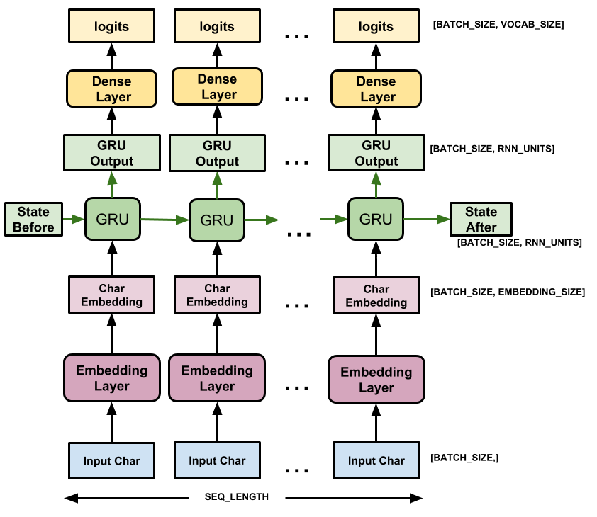
)For each character, the model looks up its embedding, processes it through a GRU unit for one time step, and then passes the output through a dense layer to generate logits that predict the log-likelihood of the next character. See image below that describes how the data passes through the model in general.
Note: The image has been sourced from the original TensorFlow tutorial about Text generation with an RNN.
Try the Model
Run the test model on one batch of input-output pairs from the dataset to verify that it behaves as expected. Check the shape of the output to start with.
# Iterate over the first batch of input-output pairs from the dataset.
for input_example_batch, target_example_batch in dataset.take(1):
    # Generate predictions for the input batch by passing it through the model.
    example_batch_predictions = test_model(input_example_batch)

    # Print the shape of the output predictions.
    print(example_batch_predictions.shape, "# (batch_size, sequence_length, vocab_size)")
Note: Since dataset.take(1) retrieves only a single batch (the first batch) of data, the unpacked variables input_example_batch, target_example_batch, and example_batch_predictions remain accessible outside the for loop. These variables will be used later in the code.
Investigate the model.
# Investigate the model.
test_model.summary()
To get actual predictions from the model, sample from the output distribution instead of simply taking the argmax of the logits and selecting the character with the highest probability (the “most likely” next character). The logits define a probability distribution over the character vocabulary for the next character. Sampling from this distribution helps select an actual character index in a way that introduces randomness into the generation process. This randomness is crucial because always using argmax can cause the model to get stuck in repetitive loops, continually predicting the same character. By sampling, the model generates different outputs each time, even when starting from the same context.
For the first example in the first batch of data, sample indices from the model’s predicted probability distribution to select the next character at each time step. Remove unnecessary dimensions and convert the result for further processing.
# Sample indices from the predicted probability distribution.
# This selects the next character based on the model's logits for the current time step.
sampled_indices = tf.random.categorical(example_batch_predictions[0], num_samples=1)

# Remove extra dimensions of size 1 from the sampled indices and
# convert the tensor to a NumPy array for easier manipulation.
sampled_indices = tf.squeeze(sampled_indices, axis=-1).numpy()
View the prediction of the next character index at each time step.
# View the prediction of the next character index at each time step.
sampled_indices
Print the input text for the first example in the first batch and the predicted text (next characters) based on the sampled indices from the untrained model’s output.
# Print the input text for the first example in the first batch.
print("Input:\n", text_from_ids(input_example_batch[0]).numpy())

print()

# Print the predicted next character based on sampled indices.
print("Next Char Predictions:\n", text_from_ids(sampled_indices).numpy())
Train the Model
The problem can now be treated as a standard classification task. Given the previous RNN state, and the input at this time step, we are required to predict the class of the next character.
Distributed Training and Parallelization
As indicated earlier, we would leverage TensorFlow’s distributed computing framework to optimize the use of computational resources and to minimize the time and cost required to train our model. Go ahead and set up TensorFlow to leverage TPU resources for distributed training.
The TPUClusterResolver connects to the TPU system, initializes it, and verifies that the TPU resources are ready and properly configured before starting the training process.
# Initialize the TPU cluster resolver to connect to the TPU system.
resolver = tf.distribute.cluster_resolver.TPUClusterResolver()

# Connect to the TPU cluster using the resolver.
tf.config.experimental_connect_to_cluster(resolver)

# Initialize the TPU system to prepare it for training.
tf.tpu.experimental.initialize_tpu_system(resolver)
Define a strategy to distribute the training across TPU cores, aiming to accelerate and optimize the training process. It is worth noting that in this particular case, distributed computing using the TPUStrategy reduces the training time by a factor of hundreds, as compared to the time required to train the model without implementing parallelization.
# Step 2: Define the distribution strategy to distribute the training across the TPU cores.
strategy = tf.distribute.TPUStrategy(resolver)
Attach a Loss Function and an Optimizer
The model needs a loss function and an optimizer for training. The standard tf.keras.losses.sparse_categorical_crossentropy() loss function is a good choice in this case. This is because it operates on the last dimension of the predictions, which contains the logits.
Additionally, since the model returns logits, set the from_logits flag.
# Define the loss function.
loss = tf.losses.SparseCategoricalCrossentropy(from_logits=True)
Calculate the mean loss for the predictions of the first batch of data and confirm the shape of the prediction tensor.
# Calculate the mean loss for the predictions of the first batch of data.
example_batch_mean_loss = loss(target_example_batch, example_batch_predictions)

# Print the shape of the prediction tensor: (batch_size, sequence_length, vocab_size).
print("Prediction shape: ", example_batch_predictions.shape, " # (batch_size, sequence_length, vocab_size)")

# Print the calculated mean loss for the predictions of the first batch of data.
print("Mean loss:        ", example_batch_mean_loss)
A newly initialized model should not be very confident in its predictions. For character prediction tasks, this means that the output logits should have similar magnitudes. If the model outputs very high or very low values for certain characters, it could signal poor initialization.
To check for any irregularities in the values of the output logits, confirm that the exponential of the mean loss is approximately equal to the vocabulary size. This is based on the idea that when the model is initialized with random weights, it should predict each character with roughly equal likelihood. In this case, the predicted probabilities for each character should be close to 1/vocabulary size. The SparseCategoricalCrossentropy() loss function calculates the difference between the predicted probabilities and the true labels. Therefore, taking the exponential of the mean loss approximates the inverse of the vocabulary size, as cross-entropy loss is related to the negative log-likelihood. If the mean loss is much higher than this value, it indicates that the model is overly confident in its wrong predictions, suggesting that the model is badly initialized.
Go ahead and compute the exponential of the mean loss to approximate the predicted probability distribution.
# Compute the exponential of the mean loss to approximate the predicted probability distribution.
tf.exp(example_batch_mean_loss).numpy()
Create and Train the Final Model
Since the test model performs as expected, go ahead and create the final / original model to be used for training. This final model will utilize the distributed training infrastructure provided by the TPU. This requires initializing and compiling the model within the scope of the TPU’s distributed training strategy – TPUStrategy. Configure the training procedure using the tf.keras.Model.compile() method to compile the model. Use tf.keras.optimizers.Adam with default arguments and the loss function.
# Define the scope for distributed TPU training using the "TPUStrategy".
with strategy.scope():
    # Initialize the "RNNModel" with specified vocabulary size, embedding dimension, and the number of RNN units.
    model = RNNModel(
        vocab_size=vocab_size,
        embedding_dim=embedding_dim,
        rnn_units=rnn_units
    )

    # Compile the model with Adam optimizer and the "SparseCategoricalCrossentropy" loss.
    model.compile(optimizer="adam", loss=loss)
Configure Checkpoints
Use a tf.keras.callbacks.ModelCheckpoint() to ensure that checkpoints are saved during training. A checkpoint saves a model’s state (weights and optimizer) during training, allowing you to resume training or use the model later without retraining.
# Directory to store the training checkpoints.
checkpoint_dir = "./training_checkpoints"

# Name of the checkpoint files.
checkpoint_prefix = os.path.join(checkpoint_dir, "ckpt_{epoch}.weights.h5")

# Create a callback to save the model weights during training.
checkpoint_callback = tf.keras.callbacks.ModelCheckpoint(
    filepath=checkpoint_prefix,  # Path to save the checkpoints.
    save_weights_only=True  # Save only the model weights, not the entire model.
)
Execute the Training
Define the number of epochs to train the data. 30 should be a reasonable number for the model to learn effectively from the data.
# Define the number of epochs to train the data.
EPOCHS = 30
Train and fit the model.
# Train and fit the model.
history = model.fit(dataset, epochs=EPOCHS, callbacks=[checkpoint_callback])
Generate Text
The goal of this work is to perform character-level prediction using an RNN and leverage that capability to generate text sequences. The simplest way to generate text with this model is to run it in a loop while maintaining and updating the model’s internal state at each time step. The image below illustrates the text generation process using sampling from the trained model.
Note: The image has been sourced from the original TensorFlow tutorial about Text generation with an RNN.
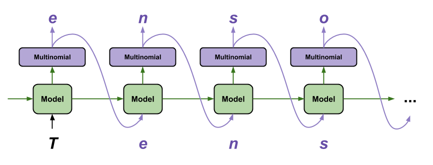
The input text and an internal state is passed to the model each time it is called. The model outputs a prediction for the next character along with an updated state. The prediction and state are then fed back into the model to continue generating text.
The OneStep class makes a single step prediction, i.e., generates one text character at each time step, taking into account the previous characters and the model state, and then predicting the next character. It takes an RNNModel and converts token IDs to characters and vice versa. The class handles sampling from the model’s predicted logits, applying temperature to control randomness, and ensuring that the [UNK] token is not selected during generation. The generate_one_step() method performs the core text generation by splitting input text into characters, running the model to predict the next character, and converting the output token IDs back into characters. It also returns the updated states, which are essential for generating subsequent characters in the sequence.
Note: To enhance performance, enable faster execution, and improve compatibility with TensorFlow, use the @tf.function decorator on the following function. Unlike eager execution, which processes operations step-by-step, this decorator converts the function into a TensorFlow graph, which is optimized and executed as a whole. Learn more.
class OneStep(tf.keras.Model):
  def __init__(self, model, chars_from_ids, ids_from_chars, temperature=1.0):
    super().__init__()
    self.temperature = temperature  # "temperature" parameter to control the randomness.
    self.model = model  # "RNNModel" for text generation.
    self.chars_from_ids = chars_from_ids  # Converts token IDs to characters.
    self.ids_from_chars = ids_from_chars  # Converts characters to token IDs.

    # Create a mask to prevent "[UNK]" from being generated.
    skip_ids = self.ids_from_chars(["[UNK]"])[:, None]  # Token ID for "[UNK]".
    sparse_mask = tf.SparseTensor(
        values=[-float("inf")]*len(skip_ids),  # Set "-inf" for the skipped token IDs.
        indices=skip_ids,  # Indices of the skipped token IDs.
        dense_shape=[len(ids_from_chars.get_vocabulary())])  # Match vocabulary size.
    self.prediction_mask = tf.sparse.to_dense(sparse_mask)  # Convert sparse tensor to dense.

  @tf.function
  def generate_one_step(self, inputs, states=None):
    # Convert strings to token IDs.
    input_chars = tf.strings.unicode_split(inputs, "UTF-8")  # Split the input text into characters.
    input_ids = self.ids_from_chars(input_chars).to_tensor()  # Map the characters to token IDs.

    # Run the model with the input token IDs and the previous state, returning both the logits and the updated states.
    # "predicted_logits.shape" is [batch, char, next_char_logits].
    predicted_logits, states = self.model(inputs=input_ids, states=states,
                                          return_state=True)
    # Only use the last prediction.
    predicted_logits = predicted_logits[:, -1, :]  # Get the logits for the last time step.
    predicted_logits = predicted_logits/self.temperature  # Adjust the logits by "temperature".
    # Apply the prediction mask: prevent "[UNK]" from being generated.
    predicted_logits = predicted_logits + self.prediction_mask

    # Sample the output logits to generate token IDs.
    predicted_ids = tf.random.categorical(predicted_logits, num_samples=1)  # Sample token IDs.
    predicted_ids = tf.squeeze(predicted_ids, axis=-1)  # Remove the unnecessary dimensions.

    # Convert from token IDs to characters.
    predicted_chars = self.chars_from_ids(predicted_ids)

    # Return the characters and the model states.
    return predicted_chars, states
Initialize the OneStep model with the trained RNN-based model and the functions to convert token IDs to characters and vice versa.
# Initialize the "OneStep" model with the trained RNN-based model and the functions to convert token IDs to characters and vice versa.
one_step_model = OneStep(model, chars_from_ids, ids_from_chars)
Run the OneStep model in a loop to generate some text. Upon investigating the generated text, it is clear that the RNN-based model understands when to capitalize, imitates dialogue-like interactions, and uses a dialogue-like writing vocabulary. However, due to the small number of training epochs, it has not yet learned to form coherent sentences or conversations and produces some misspelled words. Therefore, the model would benefit from further training.
# Start the timer to measure the execution time.
start = time.time()

# Initialize the states to "None" (no initial state for the first prediction).
states = None

# Set the initial input text for the generation (starting word).
next_char = tf.constant(["They"])

# Initialize the list of results with the starting word.
result = [next_char]

# Loop to generate text for 1000 characters.
for n in range(1000):
    # Generate the next character and update the state.
    next_char, states = one_step_model.generate_one_step(next_char, states=states)

    # Append the generated character to the list of results.
    result.append(next_char)

# Join all the characters in the list of results into one string.
result = tf.strings.join(result)

# End the timer to measure the execution time.
end = time.time()

# Print the generated text and add a separator line.
print(result[0].numpy().decode("utf-8"), "\n\n" + "_"*80)

# Print the time taken to generate the text.
print("\nRun time:", end - start)
To generate the text faster, consider batching the text generation process. For instance, in the example below, the model generates five outputs simultaneously, taking roughly the same amount of time as generating a single output in the previous example. For the complete output, see the Colab notebook for this work.
# Start the timer to measure the execution time.
start = time.time()

# Initialize the states to "None" (no initial state for the first prediction).
states = None

# Batch the text generation by providing multiple starting words at once.
next_char = tf.constant(["They", "They", "They", "They", "They"])

# Initialize the list of results with the starting word.
result = [next_char]

# Loop to generate text for 1000 characters.
for n in range(1000):
    # Generate the next character and update the state.
    next_char, states = one_step_model.generate_one_step(next_char, states=states)

    # Append the generated character to the list of results.
    result.append(next_char)

# Join all the characters in the list of results into one string.
result = tf.strings.join(result)

# End the timer to measure the execution time.
end = time.time()

# Print the entire generated text in the result, followed by a separator line to improve readability.
print(result, "\n\n" + "_"*80)

# Print the time taken to generate the text.
print("\nRun time:", end - start)
Note: Any objectionable content has been redacted in the image below.

Export the Generator
Save the single-step model and restore and use it anywhere a tf.saved_model is accepted.
# Save the "OneStep" model to the specified directory.
tf.saved_model.save(one_step_model, "one_step")

# Reload the saved "OneStep" model from the specified directory.
one_step_reloaded = tf.saved_model.load("one_step")
# Initialize the states to "None" (no initial state for the first prediction).
states = None

# Set the initial input text for the generation (starting word).
next_char = tf.constant(["They"])

# Initialize the list of results with the starting word.
result = [next_char]

# Loop to generate text for 100 characters.
for n in range(100):
  # Generate the next character and update the state.
  next_char, states = one_step_reloaded.generate_one_step(next_char, states=states)

  # Append the generated character to the list of results.
  result.append(next_char)

# Join all the characters in the list of results into one string.
result = tf.strings.join(result)

# Print the generated text.
print(result[0].numpy().decode("utf-8"))
Thoughts
We have successfully trained an RNN-based sequence model to perform character-level prediction for text generation. However, a majority of the generated sentences are not grammatically correct or coherent, though some of them are. The model has not learned the meaning of words and does tend to misspell words, but consider the following.
- The model is character-based. When training started, the model did not know how to spell an English word, or that words were even a unit of text.
- With the small number of training epochs, the model has not yet mastered forming coherent sentences or conversations and would benefit from additional training.
- Barring a few exceptions, the model knows when to capitalize text.
- Similar to the dataset, the structure of the output resembles conversations with dialogue-like text.
- Even when the model is trained on small batches of text (100 characters each), it is capable of generating longer, structured sequences of text with some degree of coherence.
Next Steps
Of course, there is a definite scope for improvement in this work. There are multiple ways to further develop this dirty implementation and improve the quality and coherence of text generated by the RNN-based model. Some of those are listed below.
- Train for Longer: Increasing the number of epochs (e.g., try setting
EPOCHS = 50) for training allows the model to learn more patterns and better representations, but be mindful of overfitting. - Experiment with Different Start Strings: Trying different starting strings could yield interesting variations and better contextual relevance in the text.
- Modify the Architecture: Adding more RNN layers – GRUs or other types of RNN layers, increasing the number of RNN / GRU units, or replacing the GRU with Long Short-Term Memory (LSTM) networks can enable the model to learn more complex patterns. Similarly, incorporating more dense (fully connected) layers can enhance the model’s capacity to capture intricate relationships. However, to prevent overfitting and manage training time and computational costs, simplifying the model architecture, rather than adding more layers, may be a more effective approach.
- Adjust
temperature: Adjusting the temperature parameter can help increase or decrease the randomness of predictions. - Hyperparameter Tuning: Experimenting with different learning rates, batch sizes, epochs, etc. can help.
- Customized Training: This tutorial adopts a simple training procedure and does not give you enough control. It uses teacher-forcing, which prevents bad predictions from being fed back to the model, so the model never learns to recover from its mistakes. Review TensorFlow’s original tutorial about Text generation with an RNN to learn more about implementing a custom training loop.
Note: You may be prompted to restart the TPU after uninstalling and reinstalling NumPy. If prompted, proceed with restarting the TPU.
Here is the link to the GitHub repo for this work.
Thank you for reading through! I genuinely hope you found the content useful. Feel free to reach out to us at ankanatwork@gmail.com and share your feedback and thoughts to help us make it better for you next time.
Acronyms used in the blog that have not been defined earlier: (a) Machine Learning (ML), (b) Artificial Intelligence (AI), (c) Random-Access Memory (RAM), (d) Tensor Processing Unit (TPU), (e) Graphics Processing Unit (GPU), (f) Identity (ID), and (g) Input/Output (I/O).