
ML and AI Blogs | Issue# 2 [July 07, 2024]
Breast cancer is one of the most common types of cancer, with early detection playing a crucial role in effective treatment and improved survival rates. This tutorial demonstrates how to build a binary classification model using TensorFlow and Keras to predict whether a breast mass is benign or malignant based on features extracted from digitized images of breast masses. The work uses a modified version of the Breast Cancer Wisconsin (Diagnostic) Data Set from Kaggle and walks through the entire ML pipeline: data loading, exploration, preprocessing, dimensionality reduction using Principal Component Analysis (PCA), model building, training, and evaluation. One may find some parts of this article about multi-class classification useful as a reference point for this tutorial.
Introduction
The goal of this tutorial is to predict breast cancer diagnosis (benign or malignant) using a DNN. This is a binary classification problem where the model predicts one of two possible outcomes. The dataset contains various features extracted from digitized images of breast masses, such as radius, texture, perimeter, area, smoothness, compactness, concavity, and more. Through this process, we will learn how to handle numerical data, perform dimensionality reduction, and build and train a neural network for classification tasks.
Setup
Begin by importing the necessary libraries.
import tensorflow as tf
from tensorflow import keras
from tensorflow.keras import layers
import numpy as np
import pandas as pds
from sklearn.decomposition import PCA
import seaborn as sns
import matplotlib.pyplot as plt
from sklearn.metrics import confusion_matrix

# Make NumPy printouts easier to read.
np.set_printoptions(precision=3, suppress=True)
Note: This work was developed using a Google Colab notebook running on a Colab-provided CPU.
Fetch and Read the Data
Load the breast cancer dataset. The dataset is a CSV file that has been downloaded and stored on Google Drive. Go ahead and import the CSV file from Google Drive.
# Import the dataset from Google Drive.
from google.colab import drive
drive.mount('/content/drive')

data_path = '/content/drive/MyDrive/Datasets/Kaggle/cancer_data.csv'
raw_dataset = pds.read_csv(data_path, na_values='?',
                         sep=',', skipinitialspace=True)
Take a quick look at the first 5 rows of the data, which includes columns for id, diagnosis (B for Benign, M for Malignant), and various features extracted from the digitized images of the breast masses, such as radius_mean, texture_mean, perimeter_mean, area_mean, and more.
dataset = raw_dataset.copy()
dataset.head()
Clean the Data
Before building the model, ensure the dataset is clean and properly formatted. First, drop features that are not important for the analysis. The id column is dropped as it is just a unique identifier and does not contribute to the prediction. The Unnamed: 32 column is also removed as it contains no relevant information.
# Drop features that are not important.
dataset.drop(['id', 'Unnamed: 32'], axis=1, inplace=True)
dataset.head()
Check for missing values.
# Check if there are missing values.
dataset.isna().sum()
Verify that there are no duplicate rows.
# Check if there are duplicate rows.
dataset.duplicated().sum()
The diagnosis column will be used as the target variable (what the model will predict). Before proceeding, convert the categorical values in the diagnosis column to binary values. A categorical feature is a variable in a dataset that represents discrete categories or groups rather than numeric values. The conversion maps B (Benign) to 0 and M (Malignant) to 1, which is more suitable for binary classification.
dataset['diagnosis'] = dataset['diagnosis'].map({'B': 0, 'M': 1})Inspect the Data
Confirm the shape of the DataFrame to understand how many samples (rows) and features (columns) are available.
# Confirm the shape of the DataFrame.
dataset.shape
Next, examine the data types. The diagnosis column should now be of type int64, and all of the other features should be of type float64, which is appropriate for a numerical analysis.
# Inspect the data types.
dataset.dtypes
Further explore the dataset and confirm it has non-null values.
# Explore the dataset further.
dataset.info()
Split the Data for Training
Divide the dataset into training and testing sets. Use 80% of the data for training and reserve 20% for testing. This split allows evaluation of how well the model generalizes to new, unseen data after training.
train_dataset = dataset.sample(frac=0.8, random_state=0)
test_dataset = dataset.drop(train_dataset.index)
Go ahead and explore the characteristics of the training data. Generate a statistical summary that can give a good understanding of the distribution of each feature.
# Explore the characteristics of the training data.
train_dataset.describe().transpose()
Next, take a look at the first five rows of the training dataset and confirm the target variable (diagnosis) and the feature columns to get a sense of what the model will be learning from.
train_dataset.head()
Separate Out the Labels from the Features
Now, separate the features (inputs) from the labels (outputs, which is the diagnosis column). Drop the target variable or feature we are trying to predict from the training and test data.
train_features = train_dataset.copy()
test_features = test_dataset.copy()

# Drop the target variable or feature we are trying to predict from the training data.
train_features_input = train_features.drop(['diagnosis'], axis=1)
train_features_labels = train_features['diagnosis'] # Training labels.

# Drop the target variable or feature we are trying to predict from the test data.
test_features_input = test_features.drop(['diagnosis'], axis=1)
test_features_labels = test_features['diagnosis'] # Test labels.
Normalization of the Training Data
Normalization is the process of rescaling input features so that they have a consistent range, typically between 0 and 1 or with zero mean and unit variance. Go ahead and normalize the input features to ensure all features are on the same scale, which helps the model converge faster during training. Use the TensorFlow Normalization layer, which standardizes features by subtracting the mean and dividing by the standard deviation.
normalizer = tf.keras.layers.Normalization(axis=-1)
normalizer.adapt(np.array(train_features_input))
dataset_normalized = normalizer(train_features_input)
print(normalizer.mean.numpy())
Compare the original and normalized versions of the first example and confirm that the values are transformed to a more uniform scale.
# Compare the original and normalized versions of the first example.
first = np.array(train_features_input[:1])

with np.printoptions(precision=2, suppress=True):
  print('First example:', first)
  print()
  print('Normalized:', normalizer(first).numpy())
Dimensionality Reduction and Feature Engineering using PCA
PCA is a statistical technique used to reduce the dimensionality of data while preserving as much of the original variance as possible. PCA works by transforming the original features into a new set of uncorrelated features called principal components, which are ordered by the amount of variance they explain.
Go ahead and use the new principal components created by PCA that are linear combinations of the original features and capture the underlying structure of the data more effectively than the original features. The Explained Variance Ratio indicates how much of the total variance in the data is explained by each principal component. The first few components typically capture most of the variance, allowing for significant dimensionality reduction.
# Perform PCA.
pca_initial = PCA(n_components=None) # Select all of the components to begin with.
dataset_pca = pca_initial.fit_transform(dataset_normalized)

# Get the Explained Variance Ratio to select the number of PCA components to use.
print("Explained Variance Ratio:")
print(pca_initial.explained_variance_ratio_)
Create a scree plot to decide on the optimal number of components for PCA. The scree plot shows the cumulative explained variance as a function of the number of principal components. This helps determine how many components to retain while preserving most of the information in the data.
# Cumulative variance of the principal components.
cum_var = np.cumsum(pca_initial.explained_variance_ratio_)

# Scree plot.
plt.plot(range(1, len(cum_var) + 1), cum_var, marker='o', linestyle='-')
plt.xlabel('Number of Components')
plt.ylabel('Cumulative Explained Variance')
plt.title('Scree Plot')
plt.show()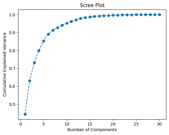
Based on the scree plot and the Explained Variance Ratio, select the number of components. Twelve components capture approximately 95% of the variance in the data, which offers a good balance between dimensionality reduction and information preservation.
# Choose number of components based on the scree plot and the Explained Variance Ratio.
num_components = 12 # 12 corresponds to approximately 95% of the Cumulative Explained Variance.
Refit PCA with the chosen number of components.
# Refit PCA with the chosen number of components.
pca_final = PCA(n_components=num_components)
dataset_pca_selected = pca_final.fit_transform(dataset_normalized)
Review the shape of the PCA-transformed data with selected components.
# dataset_pca_selected now contains the PCA-transformed data with the selected components.
print("PCA-transformed data shape with selected components:", dataset_pca_selected.shape)
Convert the PCA-transformed data into a DataFrame for easier handling. Confirm that the dimensionality is reduced from 30 features to 12 principal components, which will be used as input for the model.
# Convert the PCA-transformed NumPy array into a DataFrame for processing.
dataset_pca_selected = pds.DataFrame(dataset_pca_selected)
dataset_pca_selected.info()
Normalization of the Test Data
Apply the same normalization and PCA transformation to the test data to ensure consistency between training and testing. This ensures that the test data undergoes the same preprocessing steps as the training data, which is essential for the model to make accurate predictions on new, unseen data.
# Normalize the test data.
dataset_test_normalized = normalizer(test_features_input)

# Transform the test data.
dataset_test_pca = pca_final.transform(dataset_test_normalized)
DNN Model
Create a DNN for binary classification with the following architecture components.
- An input layer that matches the shape of the PCA-transformed features.
- Two hidden layers with 64 and 32 units, respectively, using ReLU activation functions.
- An output layer with a single unit and sigmoid activation for binary classification.
# Create the DNN model.
dnn_model = tf.keras.Sequential([
  layers.InputLayer(input_shape=(dataset_pca_selected.shape[1],)),
  layers.Dense(64, activation='relu'),
  layers.Dense(32, activation='relu'),
  layers.Dense(1, activation='sigmoid'), # For binary classification.
])
Compile the model using the following.
- The Adam optimizer with a learning rate of 0.001.
- Binary cross-entropy loss, which is appropriate for binary classification.
- Accuracy as the evaluation metric.
# Compile the DNN model.
dnn_model.compile(
  optimizer=tf.keras.optimizers.Adam(learning_rate=0.001),
  loss='binary_crossentropy',
  metrics=['accuracy'])
Investigate the model. Take a look at the prediction output which gives a preview of what the untrained model produces for the first 10 samples.
# Investigate the model.
dnn_model.summary()
dnn_model.predict(dataset_pca_selected[:10])
Set up an early stopping callback to save resources and stop training when there is no improvement in terms of minimizing the loss and improving the accuracy of the model (prevents overfitting).
early_stopping = tf.keras.callbacks.EarlyStopping(
  monitor='val_loss', # Monitor the validation loss.
  patience=5, # Number of epochs with no improvement after which training will be stopped.
  restore_best_weights=True # Restore model weights from the epoch with the best value of the monitored quantity.
)
Next, go ahead and train the model. Reserve 20% of the training data to perform validation during training.
# Fit the model with the training data.
%%time
history = dnn_model.fit(
  dataset_pca_selected,
  train_features_labels,
  epochs=200,
  batch_size=8,
  callbacks=[early_stopping],
  verbose=1,
  # Calculate validation results on 20% of the training data.
  validation_split = 0.2)
Performance Evaluation
Calculate the test loss and test accuracy of the model.
test_loss, test_accuracy = dnn_model.evaluate(dataset_test_pca, test_features_labels, verbose=2)
print(f'Test Loss: {test_loss}')
print(f'Test Accuracy: {test_accuracy}')
Plot the training and validation accuracy to visualize the learning process and to investigate if we are overfitting or underfitting the data. The history object contains information about the training process that we will leverage.
# Function to plot the training and validation accuracy.
def plot_accuracy(history):
  # Plot the training & validation accuracy values.
  plt.figure(figsize=(12, 4))
  plt.plot(history.history['accuracy'], label='accuracy')
  plt.plot(history.history['val_accuracy'], label='val_accuracy')
  plt.title('Model Accuracy')
  plt.xlabel('Epoch')
  plt.ylabel('Accuracy')
  plt.legend(['Train', 'Validation'], loc='upper left')
  plt.grid(True)
  plt.show()
plot_accuracy(history)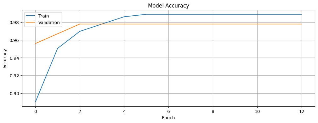
Plot the training and validation loss.
# Function to plot the training and validation loss.
def plot_loss(history):
  # Plot the training & validation loss values.
  plt.figure(figsize=(12, 4))
  plt.plot(history.history['loss'], label='loss')
  plt.plot(history.history['val_loss'], label='val_loss')
  plt.title('Model Loss')
  plt.xlabel('Epoch')
  plt.ylabel('Loss')
  plt.legend(['Train', 'Validation'], loc='upper left')
  plt.grid(True)
  plt.show()
plot_loss(history)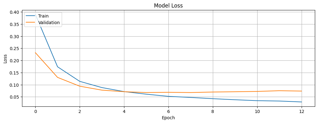
Next, generate predictions on the test set. Create a confusion matrix to evaluate the model’s performance in detail, i.e., investigate how the model performs in terms of the false positives and false negatives.
# Predict the classes.
y_pred = dnn_model.predict(dataset_test_pca)
y_pred_classes = (y_pred > 0.5).astype("int32")
# Confusion matrix.
cm = confusion_matrix(test_features_labels, y_pred_classes)

# Plot the confusion matrix.
plt.figure(figsize=(6, 4))
sns.heatmap(cm, annot=True, fmt='d', cmap='Blues', xticklabels=['Negative', 'Positive'])
plt.xlabel('Predicted')
plt.ylabel('Actual')
plt.title('Confusion Matrix')
plt.show()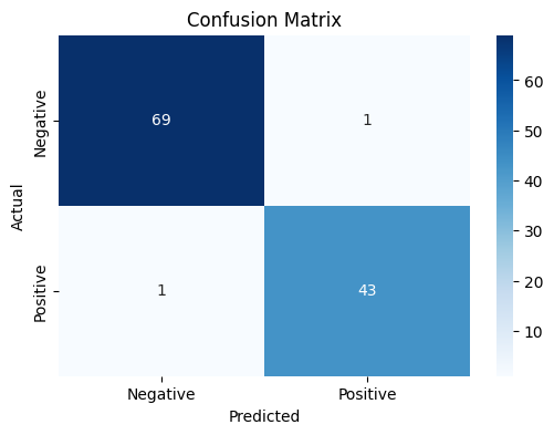
Thoughts
To achieve the goal of this tutorial – predicting breast cancer diagnosis, a DNN model was trained on breast cancer data after applying dimensionality reduction through PCA. During training, both the training and validation loss decreased steadily over the epochs, eventually plateauing, which indicates that the model learned effectively without significant overfitting.
The model achieves a test accuracy of approximately 98.25%, which is quite high for a medical diagnostic task. This means that the model correctly classifies about 98.25% of the breast masses as either Benign or Malignant based on the features extracted from digitized images.
Looking at the training and validation accuracy plot, the model quickly reaches high accuracy on both sets, with the validation accuracy stabilizing at around 97.8%, while the training accuracy continues to improve slightly, reaching close to 99%. The loss plot shows a similar pattern, with both training and validation loss decreasing rapidly in the early epochs before leveling off.
The confusion matrix provides further insight into the model’s performance. Out of the 114 test samples, there are 69 true negatives (correctly predicted Benign), 43 true positives (correctly predicted Malignant), 1 false positive (Benign predicted as Malignant), and 1 false negative (Malignant predicted as Benign). These results indicate excellent performance, with very few misclassifications.
The breast cancer prediction model demonstrates in the tutorial highlights the merit of combining dimensionality reduction techniques with deep learning for medical diagnostics. While traditional ML models might achieve good results on this dataset, the deep learning approach demonstrates strong performance, likely due to its ability to capture complex patterns in the high-dimensional data. The dimensionality reduction through PCA helps improve the model’s efficiency without sacrificing performance by focusing on the most informative aspects of the data. We are confident that learners and developers will benefit from this learning and be able to implement more sophisticated cancer classification systems by following the recommended next steps in the following section.
Next Steps
To improve the DNN-based classification model further, consider the following.
- Adding more layers or units to the neural network.
- Exploring different architectures, such as adding dropout layers for regularization.
- Experimenting with different learning rates or optimizers.
- Using ensemble methods to combine predictions from multiple models, such as Random Forests and Gradient Boosting.
- Investigating more advanced feature engineering techniques beyond PCA, such as kernel PCA or t-SNE to potentially capture additional relationships in the data that linear PCA might miss.
- Implementing cross-validation for more robust evaluation.
Here is the link to the GitHub repo for this work.
Thank you for reading through! I genuinely hope you found the content useful. Feel free to reach out to us at ankanatwork@gmail.com and share your feedback and thoughts to help us make it better for you next time.
Acronyms used in the blog that have not been defined earlier: (a) Machine Learning (ML), (b) Artificial Intelligence (AI), (c) Central Processing Unit (CPU), (d) Comma-Separated Values (CSV), (e) Rectified Linear Unit (ReLU), and (f) t-distributed Stochastic Neighbor Embedding (t-SNE).