
ML and AI Blogs | Issue# 2 [July 27, 2024]
There are multiple applications of Natural Language Processing (NLP) – the field that uses ML and AI to process and utilize language data and text. Applications include information retrieval, machine translation, language modeling, sentiment analysis, text summarization, chatbots, question-answering systems, and more. This blog will focus on solving a sentiment analysis (posed as a classification task) problem using TensorFlow.
Introduction
We will use the Sentiment140 dataset to classify the sentiment of Twitter messages using a simple neural network. While Twitter has been rebranded to X, the messages in the dataset are from 2009, when Twitter was Twitter and tweets were limited to 140 characters. We will therefore refer to X as Twitter in this work. Sentiment140 allows us to discover the sentiment of a brand, product, or topic on Twitter.
Each of the training and test data comprise of a CSV file with emoticons removed. More here.
Note: The TensorFlow dataset link does state that the labels included in the dataset are 0 (negative), 2 (neutral), and 4 (positive). However, the training dataset currently contains the labels 0 (negative) and 4 (positive). The test dataset additionally contains the label 2 (neutral), apart from 0 (negative) and 4 (positive).
Data and Computing Resources
We will first go ahead and download the data and upload it in Google Drive. Of course, we could use the local Colab environment to store the data. However, the data is roughly of 240 MB in size (~ 1.6 million tweets) and uploading the same to Colab everytime the runtime restarts or is disconnected or is reassigned is not worth the wait.
Additionally, we will require a considerable amount of computing power or RAM for processing the data (text vectorization) and for fitting the neural network model (sentiment classifier), which is not available with the free tier of Colab. We will therefore need to upgrade to Colab Pro or go for Pay As you Go, as we will need to use a GPU or a TPU to process the data and to build the model.
We will be using a TPU in this work, as it is relatively cheaper than the GPUs available in the Colab environment. That can be achieved by navigating as follows.
- Go to Runtime –> Change runtime type –> Select TPU v2 under Hardware accelerator.
We can always monitor the usage of the resources we have selected as follows.
- Go to Runtime –> View resources.
Getting Started
Let us load the relevant Python libaries.
import tensorflow as tf
from tensorflow import keras
from tensorflow.keras import layers
from tensorflow.keras.callbacks import EarlyStopping, ReduceLROnPlateau
from google.colab import drive
import pandas as pds
import csv
from sklearn.model_selection import train_test_split
import matplotlib.pyplot as plt
from sklearn.metrics import confusion_matrix
import seaborn as sns
Fetch and Read the Data
Define the paths to import the training and test data from Google Drive. Additionally, we’ll also create cleaned-up versions of our training and test data and save those in the same folder on Google Drive as the datasets.
# Import the dataset from Google Drive.
drive.mount('/content/drive')

# Define the file paths for the training data and its cleaned-up version.
input_train_file_path = '/content/drive/MyDrive/Datasets/Sentiment140/trainingandtestdata/training.1600000.processed.noemoticon.csv'
output_train_file_path = '/content/drive/MyDrive/Datasets/Sentiment140/trainingandtestdata/cleaned.training.1600000.processed.noemoticon.csv'

# Define the file paths for the test data and its cleaned-up version.
input_test_file_path = '/content/drive/MyDrive/Datasets/Sentiment140/trainingandtestdata/testdata.manual.2009.06.14.csv'
output_test_file_path = '/content/drive/MyDrive/Datasets/Sentiment140/trainingandtestdata/cleaned.testdata.manual.2009.06.14.csv'
Clean the Data
To avoid running into potential issues with the original data, we will go ahead and read the training and test data manually, line-by-line, to identify and filter out the problemactic rows and store the cleaned-up data in a new CSV file.
# Read the training and test datasets line-by-line to identify problematic rows.
# Manually filter out problematic rows and create a clean version of the CSV data file.

def clean_data(input_file_path, output_file_path):
    with open(input_file_path, 'r', encoding='ISO-8859-1') as infile, open(output_file_path, 'w', encoding='ISO-8859-1', newline='') as outfile:
        reader = csv.reader(infile)
        writer = csv.writer(outfile)

        for row in reader:
            try:
                writer.writerow(row)
            except csv.Error as e:
                print(f'Error processing row: {row}')
                continue
Let us go ahead and clean the training and test data.
# Clean the training data.
clean_data(input_train_file_path, output_train_file_path)

# Clean the test data.
clean_data(input_test_file_path, output_test_file_path)
We will now go ahead and read the new, cleaned-up training and test data.
# Read the training data into a pandas DataFrame.
raw_train_dataset = pds.read_csv(output_train_file_path, na_values='?', sep=',',
                           skipinitialspace=True, encoding='ISO-8859-1')

# Read the test data into a pandas DataFrame.
raw_test_dataset = pds.read_csv(output_test_file_path, na_values='?', sep=',',
                           skipinitialspace=True, encoding='ISO-8859-1')
Inspect the Data
Let us first confirm the size of the training and test datasets in terms of the number of examples / rows in them.
# Confirm the number of rows / examples in the training dataset.
num_examples_train = raw_train_dataset.shape[0]
print("Number of training examples:", num_examples_train)
# Confirm the number of rows / examples in the test dataset.
num_examples_test = raw_test_dataset.shape[0]
print("Number of test examples:", num_examples_test)
The next step is to investigate the cleaned-up training and test data for further analysis.
# Display the first few rows of the training dataset to verify.
raw_train_dataset.head()
# Display the first few rows of the test dataset to verify.
raw_test_dataset.head()
It can be observed by inspecting the training and test datasets that the first column contains the labels, whereas the last column houses the text (tweets) we are interested in. Let us confirm the unique values in the labels column.
# Fetch and print the unique labels in the training data.
unique_values_train = raw_train_dataset.iloc[:, 0].unique()
print(unique_values_train)
# Fetch and print the unique labels in the test data.
unique_values_test = raw_test_dataset.iloc[:, 0].unique()
print(unique_values_test)
Normalize the Data
We can observe that the training labels comprise of two values, 0 (negative) and 4 (positive). Therefore, we will now go ahead and normalize the training labels so that the 4’s are converted to 1’s (we will use 1 to denote the positive labels). This will help us when we build our model / sentiment classifier to perform binary classification.
# Normalize the training labels.
raw_train_dataset.iloc[:, 0] = raw_train_dataset.iloc[:, 0].apply(lambda x: 0 if x == 0 else 1)

# Normalize the test labels.
raw_test_dataset.iloc[:, 0] = raw_test_dataset.iloc[:, 0].apply(lambda x: 0 if x == 0 else 1)
Let us print and confirm the unique labels in the training dataset after performing normalization.
# Fetch and print the unique labels in the training data after performing normalization.
unique_values_train_normalized = raw_train_dataset.iloc[:, 0].unique()
print(unique_values_train_normalized)
It can also be observed that the test dataset is comprised of the labels 0 (negative), 2 (neutral), and 4 (positive). However, we need to ensure that the training and test data are consistent so that we can evaluate our model (a binary classifier) on the classes it was trained on. We will therefore go ahead and filter out the rows from the test dataset with the label 2 (neutral).
# Filter out the rows from the test data with the label 2 (neutral).
filtered_test_dataset = raw_test_dataset[raw_test_dataset.iloc[:, 0] != 2]
We will go ahead and take a look at the number of elements in the filtered test dataset.
# Confirm the number of rows / examples in the test dataset after filtering.
num_examples_test_filtered = filtered_test_dataset.shape[0]
print("Number of test examples after filtering:", num_examples_test_filtered)
Let us confirm the unique values in the labels column of the test data once again.
# Fetch and print the unique labels in the filtered test data.
unique_filtered_values_test = filtered_test_dataset.iloc[:, 0].unique()
print(unique_filtered_values_test)
Now that we are sure that the test data comprises of just the labels 0 (negative) and 4 (positive), we will go ahead and normalize the test labels so that the 4’s are converted to 1’s (positive labels).
# Normalize the test labels.
filtered_test_dataset.iloc[:, 0] = filtered_test_dataset.iloc[:, 0].apply(lambda x: 0 if x == 0 else 1)
Let us print and confirm the unique labels in the test dataset after performing normalization.
# Fetch and print the unique labels in the test data after performing normalization.
unique_filtered_values_test_normalized = filtered_test_dataset.iloc[:, 0].unique()
print(unique_filtered_values_test_normalized)
Separate out the Labels from the Features
Let us go ahead and extract the labels and the text data from the training and test datasets for further processing and for feeding into our model later.
# Extract the labels (first column) from the training dataset.
train_labels = raw_train_dataset.iloc[:, 0].values

# Extract the text data (last column) from the training dataset.
train_text_data = raw_train_dataset.iloc[:, -1].values

# Display the first few labels and text entries from the training dataset to verify.
print(train_labels[:5])
print(train_text_data[:5])
# Extract the labels (first column) from the test dataset.
test_labels = raw_test_dataset.iloc[:, 0].values

# Extract the text data (last column) from the test dataset.
test_text_data = raw_test_dataset.iloc[:, -1].values

# Display the first few labels and text entries from the test dataset to verify.
print(test_labels[:5])
print(test_text_data[:5])
Prepare the Data
We will now work on preprocessing the text data to be fed into our model / sentiment classifier.
Apply Text Vectorization
Next, we will standardize, tokenize, and vectorize the text data using the tf.keras.layers.TextVectorization preprocessing layer.
Standardization refers to preprocessing the text, typically to remove punctuation or HTML elements to simplify the dataset. Tokenization is the process of splitting strings into tokens (e.g., splitting a sentence into individual words by splitting on whitespace) and each token is a feature of the text data. Vectorization converts tokens into numbers so they can be fed into a neural network. All of the aforementioned preprocessing tasks can be accomplished with the TextVectorization layer.
# Maximum number of unique tokens or features to retain in the vocabulary.
max_features = 20000

# Maximum number of tokens of each input sequence / example to be processed.
sequence_length = 250

# Define the TextVectorization layer.
vectorize_layer = layers.TextVectorization(
    standardize='lower_and_strip_punctuation',
    max_tokens=max_features,
    output_mode='int',
    output_sequence_length=sequence_length)
Before proceeding with tokenization of the training and test text data, we will convert the data into strings, as the TextVectorization layer in TensorFlow / Keras expects input data to be in the string format.
# Convert all text data to strings.
train_text_data = train_text_data.astype(str)
test_text_data = test_text_data.astype(str)
Next, we will adapt the TextVectorization preprocessing layer to the training data (fit on the training data). This will cause the model to build a vocabulary – an index of strings to integers.
# Adapt the TextVectorization layer to the entire training data.
# This helps learn the vocabulary from the training data.
vectorize_layer.adapt(train_text_data)
We will now go ahead and split the training data into training and validation sets. We will use 20% of the training data for validation.
# Split the training data into training and validation data.
text_train, text_val, labels_train, labels_val = train_test_split(train_text_data, train_labels,  test_size=0.2, random_state=42)
As the final preprocessing step, let us go ahead and apply the TextVectorization layer to the training, validation, and test data, and take a look at the vectorized data.
# Apply TextVectorization to standardize, tokenize, and vectorize the training data.
text_train_vectorized = vectorize_layer(text_train)

# Visualize the training data.
print("Vectorized Training Data:\n", text_train_vectorized.numpy())
# Apply TextVectorization to standardize, tokenize, and vectorize the validation data.
text_val_vectorized = vectorize_layer(text_val)

# Visualize the validation data.
print("Vectorized Validation Data:\n", text_val_vectorized.numpy())
# Apply TextVectorization to standardize, tokenize, and vectorize test test data.
text_test_vectorized = vectorize_layer(test_text_data)

# Visualize the test data.
print("Vectorized Test Data:\n", text_test_vectorized.numpy())
As mentioned earlier, vectorization replaces each token by an integer. We can lookup the token (string) that each integer corresponds to by calling get_vocabulary() on the layer. Let us check a couple of random entries from the vocabulary and also get an idea about the size of the vocabulary.
# Check a few vocabulary entries.
print("872 ---> ",vectorize_layer.get_vocabulary()[872])
print("1729 ---> ",vectorize_layer.get_vocabulary()[1729])
print("3391 ---> ",vectorize_layer.get_vocabulary()[3391])
print('Vocabulary size: {}'.format(len(vectorize_layer.get_vocabulary())))
Configure the Data for Performance
Firstly, we will have to convert our data into a TensorFlow dataset. This step ensures efficient data handling, allows for batching, and integrates seamlessly with TensorFlow / Keras models, resulting in faster and more effective training.
# Batch size to be used for training.
batch_size = 256

# Create TensorFlow datasets.
train_dataset = tf.data.Dataset.from_tensor_slices((text_train_vectorized, labels_train)).batch(batch_size)
val_dataset = tf.data.Dataset.from_tensor_slices((text_val_vectorized, labels_val)).batch(batch_size)
test_dataset = tf.data.Dataset.from_tensor_slices((text_test_vectorized, test_labels)).batch(batch_size)
There are two important methods that should be used when loading data to make sure that I/O does not become blocking.
cache()keeps data in memory after it’s loaded off disk. This will ensure the dataset does not become a bottleneck while training the model.prefetch()overlaps data preprocessing and model execution while training.
More on both of the aforementioned methods, as well as how to cache data to disk in the data performance guide here.
# Automatically tune the buffer size for optimal data loading performance.
AUTOTUNE = tf.data.AUTOTUNE

# Cache and prefetch the datasets to improve performance.
train_ds = train_dataset.cache().prefetch(buffer_size=AUTOTUNE)
val_ds = val_dataset.cache().prefetch(buffer_size=AUTOTUNE)
test_ds = test_dataset.cache().prefetch(buffer_size=AUTOTUNE)
Build and Train the Model
We will now go ahead and define our binary classifier – a neural network model, and optimize the training process.
Define the Model
Let us define the embedding dimension for our neural network model, i.e., the length of the vector representing each word or token in the vocabulary. The embedding layer is used to transform the input tokens into dense vectors, learn the word or token representations from the training data, and to map the high-dimensional sparse input space into a lower-dimensional dense space.
# Embedding dimension.
embedding_dim = 16
We will use a simple neural network as our model for classification. Dropout will be used to regularize the model by randomly setting a fraction (30% here) of its input units to 0 during training to prevent overfitting. We will also use the GlobalAveragePooling1D layer to reduce the dimensionality of the input by averaging the features across the time steps for each training example. The final layer is a single-unit layer with a sigmoid activation function for binary classification (outputs a probability of a class or label, i.e., positive or negative sentiment).
# Define a simple neural network for the binary classifier.
model = tf.keras.Sequential([
  layers.Embedding(max_features, embedding_dim), # Configure the embedding layer.
  layers.Dropout(0.3), # Add Dropout.
  layers.GlobalAveragePooling1D(), # Reduce the input dimensions using Global Average Pooling.
  layers.Dropout(0.3), # Add Dropout.
  layers.Dense(1, activation='sigmoid')]) # Single-unit layer with a sigmoid activation function for binary classification.
# Investigate the model.
model.summary()
Select the Loss Function, Optimizer, and Evaluation Metric
The model needs a loss function and an optimizer for training. Since this is a binary classification problem and the model outputs a probability, we will use the BinaryCrossentropy loss function.
We will go ahead and configure the model to use an optimizer (Adam) and the BinaryCrossentropy loss function. Also, we will start off with a learning rate of 0.01.
Additionally, we will use `BinaryAccuracy` for the metric of our binary classifier. Given the model will output a probability, we will define a threshold of 0.5. This implies that if the probability output by the model is greater than or equal to 0.5, we will label it as 1 (*positive* sentiment), while if the probability is less than 0.5, we will label it as 0 (*negative* sentiment).
# Compile the model.
model.compile(
    optimizer=tf.keras.optimizers.Adam(learning_rate=0.001), # Pick the optimizer and the learning rate.
    loss='binary_crossentropy', # Select the loss function.
    metrics=[tf.metrics.BinaryAccuracy(threshold=0.5)]) # Choose an evaluation metric.
Define Callbacks
We will set up an EarlyStopping callback to save resources and stop training when there is no improvement in terms of minimizing the loss and improving the accuracy of the model.
# Define an early stopping callback.
early_stopping = EarlyStopping(
    monitor='val_loss', # Monitor the validation loss.
    patience=3, # The number of epochs with no improvement after which training will be stopped.
    restore_best_weights=True # Restore model weights from the epoch with the best value of the validation loss.
)
We will also use the ReduceLROnPlateau callback to monitor the validation loss and reduce the learning rate if the validation loss does not improve for a predefined number of epochs.
# Define a callback for reducing the learning rate as required.
reduce_lr = ReduceLROnPlateau(
    monitor='val_loss', # Monitor the validation loss.
    factor=0.2, # Reduce the learning rate by a factor of 0.2 if the validation loss does not improve for 'patience' epochs.
    patience=2, # The number of epochs with no improvement in the validation loss, after which the learning rate will be reduced.
    min_lr=0.0001) # Minimum learning rate.
Train the Model
Let us go ahead and train our model and fit it to the training data and validate it on the validation data.
# Number of epochs to train the data.
epochs = 20

# Train and fit the model.
history = model.fit(
    train_ds,
    validation_data=val_ds,
    epochs=epochs,
    callbacks=[early_stopping, reduce_lr],
    verbose=1)
Evaluate the Model
In this section, we will perform the following tasks.
- Evaluate how the model performs with the test data.
- Plot the loss and accuracy of the model with the training and validation data.
- Have the model classify sentiments across some unseen data that we will feed it with.
- Plot the confusion matrix to investigate the model in terms of the false positives and false negatives.
Performance on Test Data
Let us evaluate the model and see how it performs on the test data in terms of the loss and accuracy.
# Evaluate the model in terms of the loss and accuracy on the test data.
loss, accuracy = model.evaluate(test_ds)

print("Loss: ", loss)
print("Accuracy: ", accuracy)
Plot the Training and Validation Loss and Accuracy
Let us plot the accuracy and loss of the model for the training and validation data and investigate if we are overfitting or underfitting the data. The history object contains information about the training process that we will leverage.
history_dict = history.history
# Explore the information about the training process available in the 'history' object.
history_dict.keys()
# Training accuracy.
acc = history_dict['binary_accuracy']
# Validation accuracy.
val_acc = history_dict['val_binary_accuracy']
# Training loss.
loss = history_dict['loss']
# Validation loss.
val_loss = history_dict['val_loss']
# Number of epochs used for training.
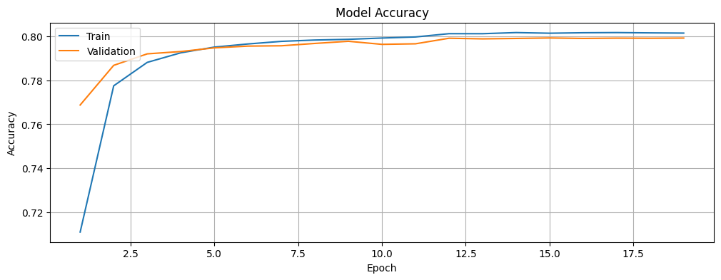
epochs = range(1, len(acc) + 1)We will now plot the training and validation accuracy of the model.
# Function to plot the training and validation accuracy.
def plot_accuracy(history):
  # Plot the training & validation accuracy values.
  plt.figure(figsize=(12, 4))
  plt.plot(epochs, acc, label='accuracy')
  plt.plot(epochs, val_acc, label='val_accuracy')
  plt.title('Model Accuracy')
  plt.xlabel('Epoch')
  plt.ylabel('Accuracy')
  plt.legend(['Train', 'Validation'], loc='upper left')
  plt.grid(True)
plt.show()plot_accuracy(history)Let us plot the training and validation loss of the model.
# Function to plot the training and validation loss.
def plot_loss(history):
  # Plot the training & validation loss values.
  plt.figure(figsize=(12, 4))
  plt.plot(epochs, loss, label='loss')
  plt.plot(epochs, val_loss, label='val_loss')
  plt.title('Model Loss')
  plt.xlabel('Epoch')
  plt.ylabel('Loss')
  plt.legend(['Train', 'Validation'], loc='upper left')
  plt.grid(True)
  plt.show()
plot_loss(history)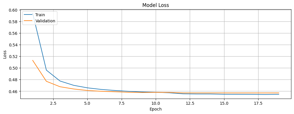
Test the Model with Unseen Data
We will feed the model with some random text examples and see how it performs.
sample_examples = tf.constant([
  "I am doing well",
  "The movie was okay.",
  "I have not been keeping well.",
  "It's a bright sunny day, let's go fishing!",
  "Great!",
  "Disaster!",
  "I am feeling confident",
  "I am not feeling confident",
])
vectorize_layer.adapt(sample_examples)
Let us go ahead and define a function that confirms whether the sentiment is positive or negative based on a threshold of 0.5, as mentioned earlier.
# Output the sentiment of the given example based on a threshold.
def interpret_predictions(predictions):
    results = []
    for pred in predictions:
        if pred >= 0.5:
          results.append("Positive Sentiment")
        else:
          results.append("Negative Sentiment")
    return results
# Vectorize the sample text examples.
vectorized_examples = vectorize_layer(sample_examples)
# Predict the sentiment of the sample text examples.
sample_predictions = model.predict(vectorized_examples)
# Interpret the predicted sentiments of the sample data.
sentiment_results = interpret_predictions(sample_predictions)
for result in sentiment_results:
print(result)
Investigate the probability values of the output predictions of the sample text examples to understand how close or off the predictions of the sentiments are.
print(sample_predictions)
Confusion Matrix
We will also plot the confusion matrix to investigate how the model performs in terms of the false positives and false negatives. Let us first get the test predictions, which are probabilities, and convert them to our labels 0 and 1 based on our threshold of 0.5.
# Predict with the test data.
test_predictions = model.predict(test_ds)
predicted_test_labels = (test_predictions > 0.5).astype("int32")
Next, we will define and plot the confusion matrix based on the labels in the test data and the labels predicted by the model.
# Confusion matrix.
cm = confusion_matrix(test_labels, predicted_test_labels)
# Confusion matrix.
cm = confusion_matrix(test_labels, predicted_test_labels)# Plot the confusion matrix.
plt.figure(figsize=(6, 4))
sns.heatmap(cm, annot=True, fmt='d', cmap='Blues', xticklabels=['Negative', 'Positive'], yticklabels=['Negative', 'Positive'])
plt.xlabel('Predicted')
plt.ylabel('Actual')
plt.title('Confusion Matrix')
plt.show()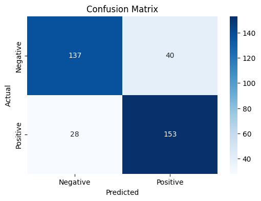
Thoughts
The model has an accuracy of about 81% and has about 40 false positives and 28 false negatives out of 358 tweets. The numbers may slightly vary across separate occasions of training. However, it is important to note that this is a quick and dirty implementation of a very simple neural network, and the results are not too bad based on the same.
It is also worth noting that while the training and validation loss decreases with time, the accuracy increases, before stabilizing and reaching a stage where there is no further noticeable improvement. Therefore, it is unlikely that we are overfitting or underfitting the data.
Next Steps
Of course, there is a definite scope for improvement in this work. There are multiple ways to further develop this dirty implementation and improve the model’s performance / accuracy for the sentiment analysis of the tweets. Some of those are listed below.
- Modifying the Architecture: Adding more layers or increasing the number of units in each layer can help the model learn more complex patterns. Using Long Short-Term Memory (LSTM or LSTMs), Bidirectional LSTMs, or fully connected / dense layers can help.
- Hyperparameter Tuning: Experimenting with different learning rates, batch sizes, epochs, etc. can help.
- Regularization: Adjusting dropout rates and the strength of L2 regularization can be used to control overfitting. Other techniques that can be used to prevent overfitting include learning rate warmup, or an advanced technique, such as label smoothing.
- Data Augmentation: Using techniques to augment the dataset can help, examples below.
- Synonym Replacement: Replace words with their synonyms.
- Random Insertion: Insert random words.
- Random Swap: Swap words in a sentence.
- Random Deletion: Delete random words.
- Pre-trained Embeddings: Using pre-trained word embeddings such as GloVe or FastText can improve the performance of the model.
- Ensemble Methods: Using ensemble methods, such as combining predictions from multiple models can improve performance.
- Fine-tuning Pre-trained Large Language Models (LLMs): Using pre-trained LLMs, such as BERT, GPT-4, or similar models from the Hugging Face Transformers library can significantly uplift the performance of word-based models.
- Hyperparameter Optimization: Using libraries, such as Keras Tuner or Optuna to find the best hyperparameters for the model.
Here is the link to the GitHub repo for this work.
Thank you for reading through! I genuinely hope you found the content useful. Feel free to reach out to us at [email protected] and share your feedback and thoughts to help us make it better for you next time.
Acronyms used in the blog that have not been defined earlier: (a) Machine Learning (ML), (b) Artificial Intelligence (AI), (c) Comma Separated Values (CSV), (d) Megabyte (MB), (e) Random-Access Memory (RAM), (f) Graphics Processing Unit (GPU), (g) Tensor Processing Unit (TPU), (h) Hypertext Markup Language (HTML), and (i) Input/Output (I/O).