
ML and AI Blogs | Issue# 1 [June 23, 2024]
Housing price prediction represents one of the fundamental challenges in real estate analytics. Accurate predictions can help homeowners, buyers, investors, and real estate agencies make informed decisions about property transactions. This tutorial demonstrates how to build a linear regression model using TensorFlow and Keras to predict house prices based on features like square footage, number of bedrooms, neighborhood, and more. We will walk through the entire ML pipeline: data loading, exploration, preprocessing, model building, training, and evaluation. TensorFlow’s tutorial on basic regression has served as a strong reference for this work.
Introduction
The goal of this tutorial is to predict housing prices using a Deep Neural Network (DNN). This is a linear regression problem where we are predicting a continuous numerical value (house price), rather than classifying into categories. This work will use a housing price prediction dataset that contains various features that might influence a house’s price, such as square footage, number of bedrooms and bathrooms, year built, and neighborhood information. Through this process, we will learn how to handle numerical and categorical data, normalize features, and build and train a neural network for regression tasks.
Note: The particular housing price prediction dataset used in this work was available on Kaggle earlier, but has since been taken down. I am happy to help if you would like to learn more about the dataset, see contact information at the end of the tutorial. However, I may not be able to share the dataset with you due to licensing restrictions. There are multiple housing price prediction datasets available on Kaggle that you might consider.
Setup
Begin by importing the necessary libraries. In particular, this work uses TensorFlow version 2.15.0.
import matplotlib.pyplot as plt
import numpy as np
import pandas as pds
import seaborn as sns

# Make NumPy printouts easier to read.
np.set_printoptions(precision=3, suppress=True)

import tensorflow as tf
from tensorflow import keras
from tensorflow.keras import layers

print(tf.__version__)
Note: This work was developed using a Google Colab notebook running on a Colab-provided CPU.
Fetch and Read the Data
Next, load the housing price prediction dataset. The dataset is a CSV file that has been downloaded and stored on Google Drive. Go ahead and import the CSV file from Google Drive.
# Import the dataset from Google Drive.
from google.colab import drive
drive.mount('/content/drive')

data_path = '/content/drive/MyDrive/Datasets/Kaggle/housing_price_dataset.csv'
raw_dataset = pds.read_csv(data_path,
                         na_values='?', comment='\t',
                         sep=',', skipinitialspace=True)
Take a quick look at the first few rows of the data. The first 5 rows of the housing price prediction dataset includes columns for SquareFeet, Bedrooms, Bathrooms, Neighborhood, YearBuilt, and Price.
dataset = raw_dataset.copy()
dataset.head()
Clean the Data
Before building our model, we need to ensure the dataset is clean and properly formatted. Check for missing values and understand the data types.
# Check if there are unknown values.
print(dataset.isna().sum())
print(dataset.dtypes)
Next, handle the categorical data in the Neighborhood column. A categorical feature is a variable in a dataset that represents discrete categories or groups rather than numeric values. Apply one-hot encoding to the Neighborhood column, which transforms this categorical feature into multiple binary columns. Each new column represents one of the possible values (Rural, Urban, and Suburb), and for each row, exactly one of these columns will have the value 1, while the others will be 0. This approach allows the neural network to properly learn from categorical features.
# Convert the categorical values in Neighborhood and numeric by one-hot encoding the values across columns for each data item.
dataset['Neighborhood'] = dataset['Neighborhood'].map({'Rural': 'Rural', 'Urban': 'Urban', 'Suburb': 'Suburb'})
dataset = pds.get_dummies(dataset, columns=['Neighborhood'])
dataset.tail()
Examine the structure of the dataset after these modifications.
print(dataset.shape)
print(dataset.info())
To ensure consistency, convert all of the numerical columns to float data type.
# Convert the Object type numerical columns to float for plotting and visualization.
numerical_columns = ['SquareFeet', 'Bedrooms', 'Bathrooms', 'YearBuilt', 'Price']
for col in numerical_columns:
  dataset[col] = dataset[col].astype(float)
  # Check for infinity values in each column.
  print(np.isinf(dataset[col]).sum())
dataset.head()
print(dataset.dtypes)
The figure below combines the information (number of unknown values in columns, shape, data types before and after conversion to float, and number of infinity values) printed about the dataset earlier.

Split the Data for Training
Now that the data is clean and properly formatted, let us split it into training and testing sets. Use 80% of the data for training and reserve 20% for testing. This split allows us to evaluate how well our model generalizes to new, unseen data after training.
train_dataset = dataset.sample(frac=0.8, random_state=0)
test_dataset = dataset.drop(train_dataset.index)
Take a look at the training dataset.
# Investigate the data.
train_dataset.head()
print(train_dataset.dtypes)
train_dataset.describe().transpose()
Inspect the Data
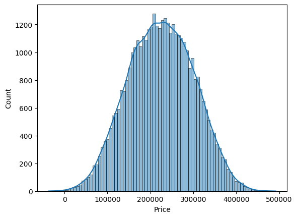
Go ahead and visualize the distribution of the numerical features to better understand the data.
for col in numerical_columns:
  sns.histplot(data=train_dataset, x=col, kde=True)
  plt.show()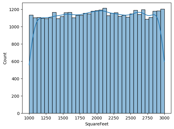
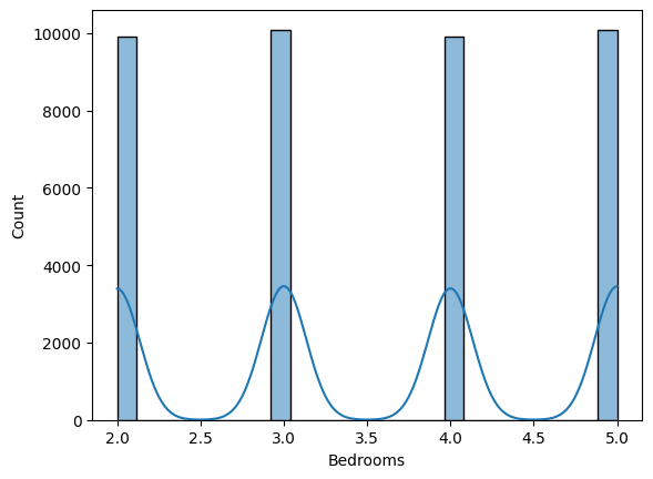
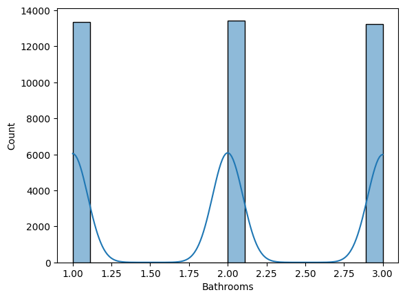
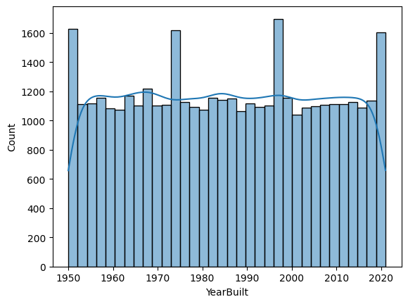
The output provides a statistical summary of the numerical features.
- SquareFeet: Ranges from 1000 to 2999 square feet, with a mean of about 2007.
- Bedrooms: Ranges from 2 to 5, with a mean of about 3.5.
- Bathrooms: Ranges from 1 to 3, with a mean of about 2.
- YearBuilt: Ranges from 1950 to 2021, with a mean of about 1985.
- Price: Ranges from –36,588 to 492,195, with a mean of about 225,056.
It is worth noting that there are some negative values in the Price column, which might need further investigation in a real-world scenario.
Additionally, the histograms reveal several insights given below.
- SquareFeet has a fairly uniform distribution between 1000 and 3000.
- Bedrooms and Bathrooms show discrete distributions, as expected for these features.
- YearBuilt shows a relatively uniform distribution from 1950 to 2020.
- Price follows an approximately normal distribution centered around 225,000.
These visualizations aid in understanding the range and distribution of the data, which is crucial for interpreting model performance and results later.
Separate Out the Labels from the Features
Next, separate the features (inputs) from the labels (outputs, which is the Price column). Create separate variables for the features and labels, both for the training and test sets. Convert everything to float32 to ensure compatibility with TensorFlow operations.
train_features = train_dataset.copy()
test_features = test_dataset.copy()

# Convert the features and labels into float so that conversions between NumPy arrays and Tensors are seamless.
train_features_float = train_features.astype('float32')
train_labels_float = train_features_float.pop('Price')
test_features_float = test_features.astype('float32')
test_labels_float = test_features_float.pop('Price')
Normalization
A crucial step in building neural networks is normalizing the input features. Normalization is the process of rescaling input features so that they have a consistent range, typically between 0 and 1 or with zero mean and unit variance. This prevents features with larger magnitudes from dominating the learning process and helps the model converge faster during training by ensuring all features are on a similar scale.
Use the TensorFlow Normalization layer, which standardizes features by subtracting the mean and dividing by the standard deviation to create the normalizer. The normalizer will be used during model training.
normalizer = tf.keras.layers.Normalization(axis=-1)
normalizer.adapt(np.array(train_features_float))
print(normalizer.mean.numpy())

first = np.array(train_features_float[:1])
with np.printoptions(precision=2, suppress=True):
  print('First example:', first)
  print()
  print('Normalized:', normalizer(first).numpy())
Regression Model
It is time to build the DNN that implements linear regression for predicting housing prices. Since we are dealing with a linear regression problem (predicting a continuous value) rather than a classification problem, the model will output a single numerical value representing the predicted price. Create the model with the following architecture components.
- A normalization layer to standardize the input features.
- Two hidden layers (dense layers represented by Dense) with 64 units each and ReLU activation functions.
- An output dense layer with a single unit (for predicting the price).
After defining the model, go ahead and compile it using the following.
- The Adam optimizer with a learning rate of 0.001.
- Mean Absolute Error (MAE) as the loss function, which measures the average absolute difference between predicted and actual prices.
dnn_model = tf.keras.Sequential([
    normalizer,
    layers.Dense(64, activation='relu'),
    layers.Dense(64, activation='relu'),
    layers.Dense(units=1)
])

dnn_model.compile(
    optimizer=tf.keras.optimizers.Adam(learning_rate=0.001),
    loss='mean_absolute_error')
Examine the model’s architecture and print the untrained model’s predictions for the first 10 training examples.
# Investigate the model.
dnn_model.summary()
dnn_model.layers[1].kernel
dnn_model.predict(train_features_float[:10])
Train the Model
Now, define a function to help monitor the training process. Train the model for 20 epochs using the training data, with 20% of that data reserved for validation during training.
%%time
history = dnn_model.fit(
    train_features_float,
    train_labels_float,
    epochs=20,
    # Suppress logging.
    verbose=0,
    # Calculate validation results on 20% of the training data.
    validation_split = 0.2)
Create a function to plot the training and validation loss. The history object contains information about the training process that we will leverage.
# Function to plot the training loss.
def plot_loss(history):
  plt.plot(history.history['loss'], label='loss')
  plt.plot(history.history['val_loss'], label='val_loss')
  plt.xlabel('Epoch')
  plt.ylabel('Error [Price]')
  plt.legend()
  plt.grid(True)
  plt.show()
plot_loss(history)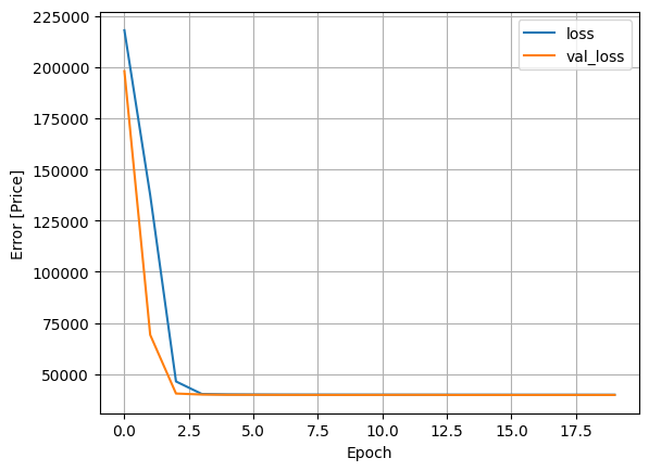
Evaluate the Model
Finally, evaluate the trained DNN model on the test dataset to see how well it generalizes to unseen data.
# Collect the test results.
test_results = {}

test_results['dnn_model'] = dnn_model.evaluate(
    test_features_float, test_labels_float, verbose=0)
Next, check the MAE of the model.
# Check the MAE of the model.
pds.DataFrame(test_results, index=['Mean absolute error [Price]']).T
To get a visual understanding of thr model’s performance, plot the predicted prices against the actual prices.
test_predictions = dnn_model.predict(test_features_float).flatten()
# Plot the predictions.
a = plt.axes(aspect='equal')
plt.scatter(test_labels_float, test_predictions, s=1, alpha=0.5)
plt.xlabel('Price [True Value]')
plt.ylabel('Price [Predicted Value]')
plt.show()
Also analyze the distribution of prediction errors.
error = test_predictions - test_labels_float
plt.hist(error)
plt.xlabel('Prediction Error [Price]')
plt.ylabel('Count')
plt.show()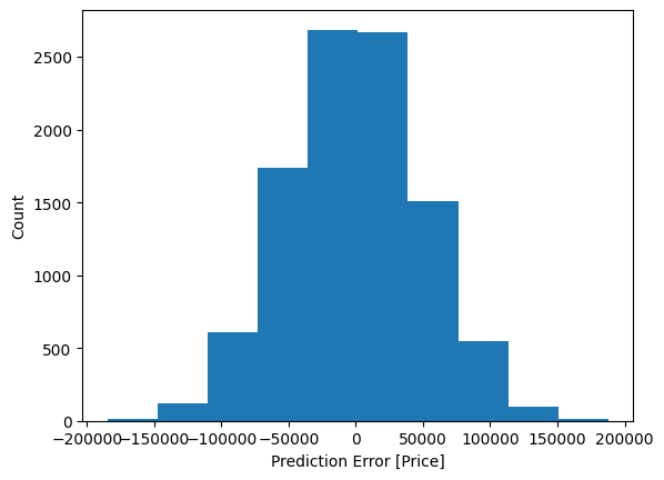
Thoughts
To achieve the goal of this tutorial – predicting housing prices, we trained a DNN model to solve a linear regression problem using housing price data. During training, the training and validation loss decreased over the epochs, declining and then starting to plateau, indicating that the model is learning effectively without significant overfitting, as we observed in the loss plot.
The model achieves a MAE of approximately 40,376.86 on the test dataset. This means that, on average, the predictions are off by about $40,376.86. Considering that the average home price in the dataset is around $225,056, this represents about an 18% average error rate.
The scatter plot of true versus predicted prices reveals that most predictions cluster reasonably close to the actual values, but there are some outliers where the model’s predictions deviate significantly. The points would ideally fall along a 45-degree line, and the spread around this line indicates the magnitude of the prediction errors.
The histogram of prediction errors further supports our analysis. It can be observed that the prediction errors (predicted price minus actual price) follow an approximately normal distribution centered near zero, which is a good sign. Most of the predictions have relatively small errors, with fewer instances of large errors in either direction.
While a traditional linear regression model might struggle with capturing complex relationships in the data, our neural network-based approach achieves reasonable accuracy for the dataset and provides a strong foundation for more advanced housing price prediction methods. The chosen architecture allows the model to effectively learn the relationships between the features and the target variable. In real-world applications, one might consider incorporating additional features, such as proximity to schools, crime rates, or economic indicators to further improve prediction accuracy. We believe that this tutorial will aid learners and developers in learning core ML concepts and in implementing more sophisticated regression-based prediction systems by following the recommended next steps in the following section.
Next Steps
To improve the DNN model, consider the following.
- Adding more layers or units to the neural network.
- Exploring feature engineering to create more informative inputs, such as creating interaction terms between related features.
- Experimenting with different optimizers or learning rates.
- Using regularization techniques to prevent overfitting.
- Trying a more complex architecture, such as adding dropout layers.
Here is the link to the GitHub repo for this work.
Thank you for reading through! I genuinely hope you found the content useful. Feel free to reach out to us at ankanatwork@gmail.com and share your feedback and thoughts to help us make it better for you next time.
Acronyms used in the blog that have not been defined earlier: (a) Machine Learning (ML), (b) Artificial Intelligence (AI), (c) Central Processing Unit (CPU), (d) Comma-Separated Values (CSV), and (e) Rectified Linear Unit (ReLU).